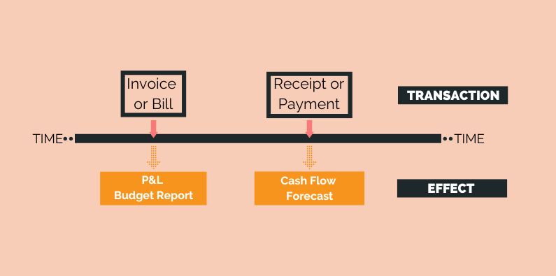
Accurate cash flow forecasts rely on getting inflows and outflows right. Timing of debtor and creditor payments are at the heart of all cash flow forecasts. How do you predict when money will be received and payments will be made? So here is how Calxa calculates the timing of debtor and creditor payments to give you an accurate future cash position.
How Does Calxa Manage Timing?
Our cashflow forecasts aren’t based on some mysterious “artificial intelligence” that you just have to blindly accept. They are founded on core accounting principles that anyone with the time and patience can follow. Yes, it’s much slower to work it all out manually but that’s why you use Calxa for your forecasts. Once you understand how it works, you can be confident in your predictions. You’ll be able to explain them to your client or to your boss. There are no mysteries in accounting.
We all know that relying on agreed payment terms isn’t realistic for predicting the future. You might dictate 30-day terms to your customers but, unless you have a direct debit authority, they won’t all pay exactly on day 30. Some will pay early, some on time. Most will probably pay late.
Calxa looks at what you currently have outstanding and then calculates a payment profile from that. This gives you an estimate based on what is actually happening. And, not what you wish was happening (though you can override the default cashflow settings).
Creditor Days and Debtor Days
Every account has a Cashflow Type. For the most part this is Creditor Days for Expense or Cost of Sales accounts and Debtor Days for Income accounts.
By reviewing the default KPI for Creditor Days, you will see that it is calculated as:
[Trade Creditors] / [Creditor Expenses] * 365
Where:
[Trade Creditors] is the combined closing balance at the Last Actuals Period for all accounts nominated in the Cashflow Forecast settings as Trade Creditors. Turn off the Advanced View if you can’t see this option.
[Creditor Expenses] includes all accounts where the Cashflow Setting indicates Creditors apply. In general, this is expense accounts that have a cashflow type set to Creditor Days or a Profile that is not set to 100% current. This group is then calculated as the sum of all movements in these accounts for the 12-month period ending the Last Actuals Period.
Debtor Days is calculated as:
[Trade Debtors] / [Debtor Income] * 365
Where:
[Trade Debtors] is the combined closing balance at the Last Actuals Period for all accounts nominated in the Cashflow Forecast settings as Trade Debtors.
[Debtor Income] includes all accounts where the Cashflow Setting indicates Debtors apply. In general, this is Income accounts that have a cashflow type set to Debtor Days or a Profile that is not set to 100% current. This group is then calculated as the sum of all movements in these accounts for the 12-month period ending the Last Actuals Period.
The end result of either of these formulas is a number which is then used to create a payment profile. The payment profile is calculated as a normal distribution (or bell-shaped curve) where the resulting day’s count is the mean (centre of the curve).
Fig 1: Example Payment Profile with Creditor or Debtor Days equal to 50
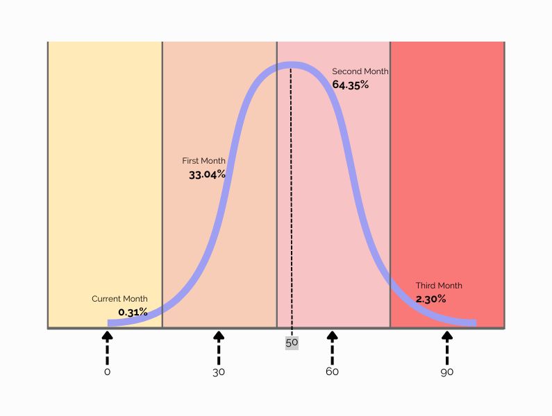
Note: For illustrative purposes only and may not be to scale.
The Payment Profile
The example above shows a payment profile that has been calculated from a days’ count of 50. The following assumptions are applied when calculating the payment profile:
- Invoices are added evenly throughout the month with the median being the middle of the month. This is why the graph starts in the middle of the current month;
- Each month is assumed to have 30 days. As a result, 30, 60 and 90 days is the middle of each month following;
- Some invoices are paid early, and some are paid late and this results in a normal distribution around the mean or average days count (50 in the case of Fig 1).
Calculating the area under the curve for each of the monthly segments provides the Payment Profile. So, in this example, we expect 0.31% of invoices issued to be paid in the same month. Followed by 33.04% to be paid in the month thereafter and so on through to the 3rd month.
Note: You can create custom payment profiles on each General Ledger account. In the rest of this article, we will refer to the payment profile. Whether this profile is manually created or auto calculated as explained above, the resulting profile is what is applied in the cashflow calculations.
Calculating the Timing of Debtor and Creditor Payments
For an example of the calculations, download this Excel Workbook titled “Debtor Example”. Here you can follow a Sales and Debtor example. But, be aware, the exact same principles are applied to Creditors. To work through the calculations, you can follow along with the workbook’s sample data and included formulas.
Note: For simplicity, we have excluded GST/VAT (Tax) in this example but in reality, GST/VAT is also being factored and added to cashflows according to each account’s Tax Code. This is generally set in the accounting system on each account in the Chart of Accounts.
Let’s set the scene
There are two sales accounts; Sales A and Sales B. Each has a separate payment profile noted at the top of the worksheet. Throughout the workbook, we will calculate the cashflows associated with a Sales Base for each of these accounts. In periods prior to and including the Last Actuals Period (in this case Feb) the Sales Base is actual sales. Whilst in periods after the Last Actuals Period, the Sales Base is budgeted sales.
Raw Cashflows
Using the Sales A Base values and the Sales A Payment Profile we can multiply out the cashflows for the current month, 1 month and 2 months.
Let’s break down the March Sales A Raw Cashflow amount of 1550. This is calculated as:
- 40% of 2000 = 800
- 30% of 1500 = 450
- 30% of 1000 = 300
The same concept is applied throughout the rest of the cashflows. Using these cashflows we can also calculate a debtors movement and, therefore, a debtors closing balance.
Note: In actuals periods the Raw Cashflow values are grey as these are theoretical values only. They do not represent actual cashflows.
Raw Unadjusted Cashflow
In a perfect world where everybody pays exactly as the payment profiles suggest then; [Debtors Movement] = [Sales A Base] – [Sales A Expected Cashflow].
In reality though, the world is not perfect and the payment profiles do not match exactly what occurs with your Debtors Movement in every month. So, in this example we are showing that; [Actual Debtor Movement] in Feb = 700 (Cell G25 highlighted is red).
We expected this to be 600 (Sales of $1,500 less receipts of $900), but for whatever reason, it just didn’t happen that way. People did not pay as expected and we now have a 1300 closing balance on debtors as opposed to 1200.
This example shows that without adjusting the cashflows we now effectively forget about this difference of 100 and we will never collect it in a cashflow forecast. If we cease trading and don’t budget sales beyond May we should expect to collect on all outstanding Debtors. This doesn’t occur because we have not adjusted for the variance in Debtors movement in the actuals period (Cell N26 highlighted in red).
Adjusted Cashflow
This example is set up in the same way with a 100 variance in Debtors for March. While this example, only includes 1 account it is easy to see that the 100 variance is attributed to Sales A. In a real-world example there are more than likely many sales accounts. Calxa does not use invoice or transaction level detail for cashflow forecasts but rather analyses the monthly movements on accounts. It calculates a statistical cashflow forecast. So if we don’t know about specific transactions how do we adjust for the debtor variance and on which accounts? This example will show how we employ an adjustment ratio.
The Adjustment Ratio
You will note there is a Debtor Adjustment Ratio (Cell G42 highlighted in green) which is calculated as [Debtor Closing Actual] / [Debtor Closing Expected]. This adjustment ratio is then applied to all cashflows that are calculated as a factor of a Sales Base Actuals period (Cells H34, H35, and I35 highlighted in green). It is only applied to these values because the variance is in the actuals balance and we, therefore, need to adjust only in the periods based on actuals.
Following the rest of this example you see we have now adjusted for the debtor variance and if we cease trading and don’t budget sales beyond May we now forecast to collect all of our debtors (Cell N38 highlighted in green).
Two Sales – Raw Unadjusted Cashflow
Building on our example with one sales account, we will now look at two sales accounts. Using a similar example, there is a variance between the actual debtor movement and the expected debtor movement (Cell G56 highlighted in red). Except, this time, as discussed earlier, we really don’t know which sales account the variance is related to. Just as with the original example if we don’t adjust the cashflows then we will never correct the variance in the actuals debtors balance (Cell N57 highlighted in red).
Two Sales – Adjusted Cashflow
Whether you have one sales account, two sales accounts or many sales accounts the exact same logic is applied to adjust the raw cashflow amounts.
- First of all we calculate an adjustment ratio (Cell G78 highlighted in green) which is calculated as [Debtor Closing Actual] / [Debtor Closing Expected].
- This adjustment ratio is then applied to all the cashflow amounts that are a factor of Actuals periods. The adjustment ratio is not applied to cashflows calculated as a factor of budgeted periods. In this example, there are 6 cells that have the adjustment ratio applied (Cell H66, H67, I67, H70, H71, I71).
As you can see the adjusted cashflow figures now wash out the debtor variance. And, if we stop budgeting beyond May, all debtors are collected.
Discussion About the Adjustment Ratio
Under normal circumstances, the adjustment ratio will be quite small (close to 1). However, if your cashflow profile does not match reality, your cashflow forecast may yield strange looking results. It could be influenced by large inflows or outflows in the first few months.
Realistic Cashflow Settings
For example, if all your income accounts have a custom profile of 100% in month 1 or you override the debtor days value to 30 days, then you are telling Calxa that all your outstanding debtor income will be collected in the first month.
Another way to look at it is that you are telling Calxa your forecasted closing debtors for the current month will be whatever you budget for this month. Imagine your average monthly sales are $50,000 but your outstanding debtors are $100,000. The first month in your cashflow will collect the full $100,000. But, you might be asking why your inflows are so high when you only did $50,000 sales last month. The problem here arises because the cashflow settings don’t match reality. It is not realistic to say you collect all your income in the first month if there is $100,000 in outstanding debtors but you only invoiced $50,000 last month. Generally, this problem will not occur if you are using default cashflow settings.
One-Off Large Invoices
Another thing to understand about the adjustment ratio is that it is accounting for values that sit outside the payment profiles by adjusting all cashflows, not just the account that has the outstanding invoice. The intention of this type of adjustment is to make your overall inflows or outflows as accurate as possible but not to highlight exactly which account has outstanding invoices. This is most noticeable if you have a large transaction and you are expecting to see this large transaction in the cashflow show up on a specific account.
Now let’s imagine this large income transaction ($100,000) was invoiced two months ago and we have similar cashflow settings to above, where everything is set to 100% in month 1. The outstanding amount will not be picked up by the raw cashflow values. This is because it is outside the 100% month 1 scope. Instead, the adjustment ratio will now pick up the variance in the debtors’ balance. It will apply it to all debtor inflows. It is important to understand that the $100,000 is still accounted for. However, the inflows are now spread across all your debtor income accounts instead of the one account.
Test Your Timing of Debtor and Creditor Payments
If you have used the workbook from this article to calculate the Timing of Debtor and Creditor Payments. Maybe the next step is to try Calxa to see how easy it is to produce your cash flow forecast. Sign Up for a free trial and have a go.